Chapter 11 REASONING AND ASPECTUAL-TEMPORAL CALCULUS Jean-Pierre Descl´es University of Paris-Sorbonne
In the present a...
18 downloads
825 Views
1009KB Size
Report
This content was uploaded by our users and we assume good faith they have the permission to share this book. If you own the copyright to this book and it is wrongfully on our website, we offer a simple DMCA procedure to remove your content from our site. Start by pressing the button below!
Report copyright / DMCA form
Chapter 11 REASONING AND ASPECTUAL-TEMPORAL CALCULUS Jean-Pierre Descl´es University of Paris-Sorbonne
In the present article, we propose a formal representation of the reasoning expressed in and by natural language sentences like: (1) The hunter has killed the deer. therefore: 1/ The deer has been killed. 2/ The deer is dead. 3/ The deer is no longer alive. 4/ The deer had been alive. (2) Peter has come out of the garage. therefore: 1/ Peter was in the garage. 2/ Peter is no longer in the garage. 3/ Peter has come outside the garage from the inside. (3) Peter is already back home. therefore: 1/ Peter was not at home sometime earlier. 2/ One could expect that Peter was not at home. (4) If Peter had been there, Mary would not have left. 1/ Since Peter was not there, Mary has left. D. Vanderveken (ed.), Logic, Thought & Action, 217–244. 2005 Springer. Printed in The Netherlands.
c �
218
LOGIC, THOUGHT AND ACTION
(5) One more step and I will shoot. therefore: 1/ You have the intention of making one more step. 2/ I don’t shoot but I have the capacity of shooting. How can we infer the sentences (1.1), (1.2), (1.3) and (1.4) from (1)? What are the operations we must execute from the understanding of aspectual and temporal grammatical markers and from the understanding of lexical units? The same questions can be asked about (2), (3), (4) and (5).
1.
Theoretical Framework
In order to explain this kind of problem, one has to be able to build metalinguistic representations of the above sentences in a way that such inferences are automatic. The formal model of the metalinguistic representations that we choose is applicative (or functional), which means that it applies operators to different types of operands (Descl´ ´es, 1990). These applicative representations take Church’s lambda-calculus applicative formalisms with types, as well as Curry’s (1958) (see Appendix) Combinatory Logic with types. Since the above reasoning requires aspectual and temporal notions, we will use actualization intervals associated with predicates and sentence relations (that means the intervals of instants between which a predicative relation is considered as actualized or true). Indeed, the analyses of aspects and tenses that we have presented in different publications is based on topological representations (Descl´´es, 1980, 1990b, 1991, 1993; Guentcheva, ´ 1990; Maire-Reppert, Oh, Berri, 1993; Descles ´ & Guentch´´eva, 1990, 1995. . . ). Therefore, we attach topological operators interpreted on topological intervals of instants. We associate with an interval of instants two boundaries : a left boundary γ(I) and a right boundary δ(I). A boundary of a topological interval can be “open” (in this case, the boundary does not belong to the interval) or can be “closed” (in that case, the boundary belongs to the interval). An interval is closed when its left and right boundaries are closed; it is open when its left and right boundaries are open; it is semi-open when its left boundary is closed and its right boundary is open. The knowledge of lexical meanings (verbs in particular) requires knowledge of representation formalisms such as Sowa’s conceptual graphs. As far as we are concerned, we use the representations such as the semanticcognitive schemes which we have presented in several previous publications (Descl´´es, 1990a, 1994, Abraham, 1995). Each of these schemes represents the meaning of a predicate by a typed λ-expression.
Reasoning and Aspectual-Temporal Calculus
219
We have indicated that the applicative metalinguistic representions constitute a formalism on the basis of combinatory logic and λ-calculus. Combinatory logic with types was used for analysing grammatical problems such as passivization, reflexivization, typology of voices (Shaumyan, 1987; Descl´´es, Guentch´eva, Shaumyan, 1985,1986; Descl´es, 1990). We will argue here that this formalism is adequate to analyse the reasoning in natural languages by means of reductions (technically β-reductions). The method of this formalization is divided into several phases: 1/ Observation and analysis of linguistic data; 2/ Conceptualization by means of a concept network (for example, concerning all aspects: process, event, state, perfect, perfective, imperfective. . . ); 3/ Schematization and design of the schemes (for example, the use of semantic-cognitive schemes for the representation of predicate meanings); 4/ Mathematization of concepts, operations and intuitive schemes (for example, the use of topology and basic operations such as application); 5/ Construction of a formal language that must be adequate to formalize the intuitive conceptualizations; 6/ Interpretation of this formal language in a model (Tarski’s sense). Instead of starting from a pre-established formal language (such as, for example, Prior’s tense logic), we prefer defining and interpreting a formal metalanguage, this starting from a more or less mathematized model. This approach implies a conceptualization of intuitive notions (for example: progressivity, perfectivity, inchoativity. . . ), which we will later try to formulate in a mathematical way. Many of the logicians (such as, for example, in Montague’s approach) start from formal languages (a logic of tenses, a logic of modalities or a logic of indexical terms), and then build corresponding semantic models in order to provide to a certain extent approximations of natural languages. We take the opposite approach: first, we define the model which has already been mathematized (for example, a quasi-topological model of states, events and process or a model of speech-act operations); second, we express the concepts of the model in terms of operators of combinatory logic. This formal language is a metalanguage in the way it describes the semantics of grammatical categories of natural languages.
220
LOGIC, THOUGHT AND ACTION
The theoretical framework in which we develop the following linguistic analyses is that of the Cognitive Applicative Grammar which can be regarded on the one hand as an extension of Shaumyan’s Universal Applicative Grammar (1987) with integrations of cognitive representations, and on the other hand as formalizations of speech-act operations from the works of Benveniste (1964), Searle and Vanderveken (1985) and Culioli (1994). In the Cognitive Applicative Grammar (Descl´ ´es, 1990a), there are three different representation levels with explicit processes of change of representations from one level into another. These three levels are: (i) the level of phenotype representations — or morpho-syntactic configurations -, its task is the analysis of the morpho-syntactic data of different languages; (ii) the level of genotype representations — or logico-grammatical operations -, its task is to exhibit the invariants and the grammatical functions of language; (iii) the level of semantic-cognitive representations, its purpose is, first, the analysis and the formal representations of the meanings of lexical units, and second, the interaction of language activities with other cognitive activities of human perception and action. The change of representations from one level into another is similar to the generalized compiling process of high-level programming languages. This compiling process changes units from one representation level to another by means of synthetical “reunitarization” (definition of new units from given units) or by means of analytical “decompositons” of a unit. This device is oriented by an “intelligent” mechanism called “contextual exploration”. The purpose of this mechanism is to resolve ambiguities by locating the relevant contextual information during different stages of the process, thus orienting the process towards a decision for solving ambiguities in some grammatical units. The goal of this complex device (compiling directed by contextual exploration) is to establish an explicit relationship between abstract representations and directly observable linguistic configurations.
2.
Conceptualizations of Aspect and Tense
We recall some of the theoretical elements of the aspect-tense model that we have developed and presented in several previous publications. A predicative relation λ or “propositional content” (which is called a “lexis” by Culioli (1994)) is organized by means of predicate operations.
221
Reasoning and Aspectual-Temporal Calculus
These predicate operations are very well analyzed and expressed in an applicative formalism. We can consider the following applicative expression with prefixation of the predicate operator: (*)
“to see” “a-deer” “the-hunter”
This applicative expression is obtained by means of two successive applictive operations. First, the predicate “to see” is an operator that applies to a first operand “deer”; the result is a new operator that applies to a second operand “hunter”. The result is the predicative relation (*). The building of this predicative relation is represented as follows: “to see” “to see” “a-deer”
“a-deer” > “the-hunter” >
“to see” “a-deer” “the-hunter”
Such a predicative relation is tenseless. Before inserting it in a reference space, the speaking subject perceives it in different ways, depending on whether he views it as a progressive process, an event or a resultative state. Thus the subject constructs an aspectualized predicative relation (Descl´´es, 1991) which is considered as true on a topological interval of instants I. We note this aspectual predicative relation as follows: (**)
ASP PI (“to see” “a-deer” “the-hunter”)
where the aspectual operator ASP applies to the predicative relation (*). According to whether the aspect is a state, an event or a process, the interval I will be respectively open, closed or semi-open. We say that the state, the event or the process is true (or actualized) on this topological interval I. Having aspectualized the predicative relation, the subject now has to insert it into his own time reference that is distinct from the external time reference (the clock time, the cosmic time, the calendar time. . . ). The subject will or will not consider the aspectualized predicative relation as concomitant with his own process of speaking, that cannot be reduced to a punctual instant because each process of speaking takes time. In this reference, T0 denotes “this first non-actualized instant”, which means the right boundary (unfinished) of the speaking process in progress (Descl´´es, 1980, 1990b, 1994; Descl´ ´es & Guentch´eva, 1990, 1995). We have therefore several sentences with the same propositional content (*), for example: (a) The hunter is looking at the deer at this moment (Unfinished) process concomitant with the speaking process in progress
222
LOGIC, THOUGHT AND ACTION
(b) Finally; the hunter has seen the deer, he is happy Resultative state of a finished anterior process (c) While the hunter was looking at the deer (Unfinished) process non concomitant with the speaking process in progress (d) The hunter saw the deer, and then he Event inserted into a series of events With topological representations (which means the diagrams of the actualization of the aspectual predicative relation (**) in accordance with a choice of different aspectual and temporal scope), we will have respectively the differents temporal diagrams given in figure 1. (a’) (b’)
(c’) (d’)
-------------[ [T0 [T0 --[----------] � [T - - - [T0 --[ ] - - - - - - - - - - [T0 --[ Figure 1.
In a general way, an aspectualized predicative relation ASP I (Λ) will be actualized (or realized) on an interval I. If this relation is aspectualized as a state, or respectively as an event or as an unfinished process, it will be true respectively on an open interval O, on a closed interval F or on an interval J closed at the left boundary and open at the right boundary (Descl´´es 1990b). When I designates an interval (open or closed or semiopen), γ(I) and δ(I), the respective bounds are the left or the right of the interval I. If an interval is open, then the two bounds (at left and at right) do not belong to the interval. If the interval is closed, then the two bounds (at left and at right) belong to the interval. We have thus the three diagramatic representations of realization intervals according to the aspects of the predicative relations: a state, an event and an (unfinished) process. We have three more specific aspectual operators STATE, EVENT and PROC. C The intervals, with topological boundaries, where the aspectualised predicative relations are realized are shown by temporal diagrams (see figure 2): Remark: We consider (Descl´´es, 1980, 1995; Decl´´es & Guentcheve, 1995), the trichotomy state / event / process essential in the analy-
223
Reasoning and Aspectual-Temporal Calculus ]
[ STATEO (Λ)
[ ] EVENT F (Λ)
[
[ PROC J (Λ)
Figure 2.
ses of aspects in natural languages (see also: Lyons (1977), Comrie (1979) or Mourelatos (1981)). Note that this trichotomy is different from Vendler’s classification of “state”, “activity”, “accomplisment” and “achievement”. Some authors (for instance: Smith (1991), KoceskaToscewa and Mazurkiewicz (1994), Karolak (1997), Kamp (1981, 1983), Vet (1995)) claim that the dichotomy state / event (punctual) is sufficient. However, several arguments against this theoretical viewpoint have been given (see Descl´´es and Guentch´eva, 1995)). We formulate different rules about states, events and processes. 1/ RULE on STATE: IF a state STATE O (Λ) relating to a predicative relation Λ is true on an open interval O, THEN for each sub-interval O’ of O, the state relating to the same predicative relation Λ remains true over O’: ST AT EO (Λ) & [O ⊃ O� ] ⇒ ST AT EO� (Λ) Remark: One finds a similar rule in Dowty (1979). 2/ RULE on EVENT: IF an event EVEN F (Λ) relating to a predicative relation Λ is true, THEN the predicative relation Λ is true at the right boundary δ(F): EV EN NF (Λ) ⇒ (Λ)δ(F) In general, an event is actualized only at the right boundary δ(F), which is the final boundary of the event actualized on a closed interval F. The same event relating to the same predicative relation Λ is not actualized at the right boundary of each of the sub-interval F’ of F, but only at δ(F). An event will only be true if the final instant δ(F) is reached. For example, the sentence John wrote a letter in one hour is a predicative relation which is true at its right boundary (final boundary) of a closed interval F, while this predicative relation is not true in a closed subinterval F’ of F. However, in some cases, an aspectualized predicative relation Λ, viewed as an event, can be true both for a closed interval F and for each sub-interval F’ of F. An example of this case is: John ran in the park yesterday afternoon.
224
LOGIC, THOUGHT AND ACTION
3/ RULE on PROCESS: IF an unfinished process PROC J (Λ) relating to a predicative relation Λ is true on a semi-open interval J, THEN for each semi-open interval J’ with the same beginning of J (γ(J) = γ(J’)), the predicative process PROC J � (Λ) relating to the same predicative relation remains true for J’: CJ� (Λ) P ROC CJ (Λ) & [J ⊃ J� ] ⇒ P ROC Remark: for the justification of this rule, see Descl´ ´es and Guentch´eva (1995). 4/ RULE on PROCESS: IF an unfinished process PROC J (Λ) relating to a predicative relation Λ is true on an interval J, THEN when the process is finished (in French: “achev´ ´e”), it generates: (i) an event EVEN F (Λ) (relating to the same predicative relation Λ); this event is realized on a closed interval F which includes the smaller closed interval cl(J) including J, called the closure of J; (ii) a resultative state RES-STATE O (Λ) (relating to the same predicative relation Λ) which is true on an open O that is posterior and adjacent to the interval F: PROC J (Λ) ⇒ there is an EVEN F (Λ) and a RES-STATE O (Λ) such that [F ⊃ cl(J)] & [O is adjacent to F and posterior to F]
We represent this rule with the diagram of the figure 3. [ - - - - - - - - J - - - - - - - - - - >[ [ - - - - - - - - - cl(J) - - - - - - - - ] [ - - - - - - - - - - - F - - - - - - - - - - - - ]< - - - - - - - - O - - - - - - - - >[ Figure 3.
Remark: This rule is designed to capture the meaning of “perfect” in Indo-European languages (see Descl´´es, 1980; Guentch´eva, 1990).
3.
Analysis of Tenses and Aspects Let us start with the following sentence: (6)
The hunter is looking at the deer (at this moment).
The underlying logical form of the sentence is analyzed in the following steps: (i) Formation of an underlying predicative relation expressed by an applicative notation: ((“to see” “a-deer”) “the-hunter”) ; (ii) Aspectualization of this predicative relation as an unfinished process in
Reasoning and Aspectual-Temporal Calculus
225
progress, with the aspectual process operator PROC ; (iii) Inclusion of this process, called predicative process, into the speaking process in progress; (iv) Establishment of a concomitance relation between the unfinished speaking process and the unfinished predicative process. Generally, a predicative relation Λ that is viewed as an unfinished process is true on an interval J1 of instants, hence the process operator PROC J 1 and the predicative process PROC J 1 (Λ). This predicative process becomes an argument of the metalinguistic speaking predicate “SAY(. . . )S 0 ”, where the symbol S 0 denotes the abstract subject “EGO” of any speaking act: EGO is the origin of the system of persons (I, YOU, HE / SHE) as well as deictic spatial markers as HERE, THERE. The speaking process is true on the interval J0 of instants, hence the aspectual operator PROC J 0 and the following speech-act scheme (see Descl´´es, 1980): (***)
P ROCJ0 (SAY(. . .)S 0 )
Now we can express explicitly the underlying logical form of sentence (6). To simplify the notations, we use the symbol P2 to designate the transitive lexical predicate associated to the verb “to see” and respectively the symbols T1 and T2 for the terms “the hunter” and “the deer”. Formula (7) is an aspectual-tense representation of (6), expressed by a prefixed applicative notation: (7)
& (P ROCJ0 (SAY(P ROCJ1 (P2 T2 T1 ))S 0 ) ([δ(J1 ) = δ(J0 )])
This formula is a conjunction of the two constituents (7a) and (7b): (7a)
(P ROCJ0 (SAY(P ROCJ1 (P2 T2 T1 ))S 0 )([δ(J1 ) = δ(J0 )])
(7b)
[δ(J1 ) = δ(J0 )]
The predicative process PROC J 1 (P2 T2 T1 ) is in this way considered as being true on the interval J1 . Formula (7a) represents the embedding of the predicative process PROC J 1 (P2 T2 T1 ) into the speech-act process. Formula (7b) expresses a temporal constraint on the intervals of actualization of the two processes: In an unfinished process concomitant with the speech-act, the right boundaries δ(J1 ) of J1 and δ(J0 ) of J0 must be identical. Formula (7) can be read as follows: (7’)
“The speaking process “S 0 SAY. . . ”, which is true on an interval J0 , has as its argument a predicative process “P2 T2 T1 ” which is true on an interval J1 , with the temporal constraint that the two right boundaries of the two intervals J0 and J1 must be identical”
or, in others words:
226
LOGIC, THOUGHT AND ACTION (7”)
“the predicative relation “P2 T2 T1 ” is conceived from an aspectual point of view as an unfinished process which is an argument of the speaking process “S 0 SAY that. . . ”, the final sections of the two processes are identical.”
Now, we are going to define an aspectual operator by integrating the two elementary process operators PROC J 0 and PROC J 1. into a complex operator. The predicative relation “P2 T2 T1 ” becomes an argument of this complex operator. With this aim, we use the combinators B, B2 and C of the combinatory logic (see Appendix). We present the integration as in Gentzen’s “natural deduction” style but with “reunitarization” relations (or definitions of new units from an applicative combination of differents more primitives units). Thus, in the following integration process, step 9. expresses a reunitarization relation: the complex operator SA is defined in terms of the operator SAY and the operand S 0 .
Integration of the operator “Speech-act” (SA) The symbol SA designates, in the following integrative process, an operator which means that “S 0 performs a speech-act”. We call it an “enunciative operator”. 1. 2. 3. 4. 5. 6. 7. 8. 9. 10. 11. 12. 13.
P ROCJ0 (SAY(P ROCJ1 (P2 T2 T1 ))S 0 ) B2 P ROCJ SAY(P ROCJ1 (P2 T2 T1 ))S 0 C(B2 P ROCJ0 SAY)S 0 (P ROCJ1 (P2 T2 T1 )) C(CB2 SAYP ROCJ0 )S 0 (P ROCJ1 (P2 T2 T1 )) BC(CB2 SAY)P ROCJ0 S 0 (P ROCJ1 (P2 T2 T1 )) B(BC)(CB2 )SAYP ROCJ0 S 0 (P ROCJ1 (P2 T2 T1 )) C(B(BC)(CB2 )SAY)S 0 P ROCJ0 (P ROCJ1 (P2 T2 T1 )) B(C(B(BC)(CB2 ))SAYS 0 P ROCJ0 (P ROCJ1 (P2 T2 T1 )) [SA =def B(C(B(BC)(CB2 )SAYS 0 ] SAP ROCJ0 (P ROCJ1 (P2 T2 T1 )) B(SAP ROCJ0 )P ROCJ1 (P2 T2 T1 ) BBSAP ROCJ0 P ROCJ1 (P2 T2 T1 ) (SA0P ROCJ0 0P ROCJ1 )(P2 T2 T1 )
hyp intB2 intC intC intB intB intC intB def of SA repl, 8, 9 intB intB def of 0, 12
Comments: In step 1., it is shown that the predicative process is being embedded into the speech-act process; the first process is true on one interval J1 and the second is true on another J0 . Steps 2. to 8. introduce the combinators B, B2 and C which allow a combination of the speaking operators, hence the definition introduced in step 9. of the operator SA which means “the speaker performs a speaking-act” or “the speaker S 0 says that. . . ”. We deduce from the definition given at step 9., the expression given at step 10. by remplacement of the definiens. By combining the operators SA, PROC J 0 and PROC J 1 , we obtain a new complex operator (at step 12. or, equivalently, at step 13.) whose operand is P2 T2 T1 . The operators SA, PROC J 0 and PROC J 1
Reasoning and Aspectual-Temporal Calculus
227
are combined as compositions of functions. From this integrative process it follows that step 13 is an applicative integration of step 1. with the same meaning. The expression at step 13. is deduced from the expression given at step 1. At step 13., it is shown that the complex operator, “(SA 0 PROC J 0 0 PROC J 1 )” is a grammatical operator whose meaning is only aspectual. This applies to the predicative relation “(P2 T2 T1 )”. The two formulas in step 1. and step 13. are considered as being equivalent to the same aspectual meaning.
In the above deduction, we introduce a derived operator SA. Its meaning is: “the speaking subject S 0 says that”. We call it an “enunciative operator”. This enunciative operator is built by means of an application of the abstract operator (a derived abstract combinator) to the elementary operator (saying) and to the operand S 0 . Its formal definition is given by the following relation between a definiendum (at the left) and a definiens (at the right): (8)
[SA =def B(C(B(BC)(CB2 )SAYS 0 ]
At the end of the above reduction, the applicative expression obtained at step 13. represents the result of the application of a complex aspectual operator on the predicative relation (P2 T2 T1 ), that is to say: (9)
(SA 0 P ROCJ0 0 P ROCJ1 )(P2 T2 T1 )
Now, we return to the expression (6) again. We substitute in (7) the expression (7a) by (9), since the two expressions (7a) and (9) are equivalent to the same aspectual meaning, hence the expression (10): (10)
& ((SA 0 P ROCJ0 0 P ROCJ1 )(P2 T2 T1 ))([δ(1J ) = δ(0J )])
Thus, we can continue the reduction process in such a way as we define an integrated aspectual operator considered as a reunitarized operator. The operand of the first aspectual operator is a predicative relation but the operand of the second aspectual operator is a lexical predicate.
Integrative process of the verbal aspectual operator. 1. 2. 3. 4. 5. 6. 7. 8. 9.
&((SA 0 P ROCJ0 0 P ROCJ1 )(P2 T2 T1 )) ([δ(J1 ) = δ(J0 )]) C&([δ(J1 ) = δ(J0 )]) ((SA 0 P ROCJ0 0 P ROCJ1 )(P2 T2 T1 )) B(C&([δ(J1 ) = δ(J0 )]) (SA 0 P ROCJ0 0 P ROCJ1 ) (P2 T2 T1 ) (C&([δ(J1 ) = δ(J0 )])) 0 (SA 0 P ROCJ0 0 P ROCJ1 )(P2 T2 T1 ) [UNF-PRST =def (C&([δ(J1 ) = δ(J0 )])) 0 (SA0P ROCJ0 0 P ROCJ1 )] UNF-PRST (P2 T2 T1 ) B2 UNF-PRST P2 T 2 T 1 [prog-prest =def B2 UNF-PRST] T (prog-prest P2 ) T2 T1
hyp intC intB def 0 def from 5 int B2 def from 8
228
LOGIC, THOUGHT AND ACTION
Comments: step 1. has exactly the same meaning as in expression (2). The temporal constraints have been added to the proper aspectual conditions. We rearrange the operators so as we can isolate the predicative relation (steps 2 to 4). At step 4. the two operators are combined as two composed functions. Then we introduce the definition of a grammaticalized aspectual-temporal operator “Unfinished-Present”, designated by UNF-PRST at step 5. At step 6., we isolate the two arguments of the predicative relation so that we can define an operator which applies only to the predicate, hence the definition of a verbal progressive present operator designated as prog-prest at step 8. and in the final expression at step 9. The operator prog-prest is the morphological trace of the deep grammatical operator UNF-PRST which (i) encodes the temporal constraints (that two intervals of actualization have the same right boundary) and also (ii) combines the two process operators with the enunciative predicate SA. Now, the predicate P2 becomes an argument of the morphological operator prog-prest, hence the “aspectualized and tensed” new predicate “prog-prest P2 ” derived from the lexical predicate P2 .
Finally, we obtain the expressions (11) and (12) which are equivalent to the expression (7); these two expressions have the same meaning as the expression (7): (11)
UNF-PRST(P2 T2 T1 )
(12)
(prog-prestP2 )T2 T1
We remark that the grammatical operator UNF-PRST takes the entire predicative relation (P2 T2 T1 ) as its operand whereas the verbal progressive present operator prog-prest takes only the lexical predicate P2 as its operand. Now we look at the sentence (6) The hunter is looking at a deer (at this moment). This sentence can be analyzed by means of the prefixed applicative expression (6’): (6’)
is-looking-at a-deer the-hunter
The verbal operator is-looking-at can be analyzed as a complex binary predicate, derived from a lexical predicate “look-at” by means of the morphological operator “progressive present” prog-prest. Thus we have the following definition: (6”)
[is-looking-at = prog-prest look-at]
From this definition we can deduce relations between a linguistic configuration The hunter is looking at a deer expressed at the phenotype level and the corresponding applicative expressions:
Reasoning and Aspectual-Temporal Calculus (6”’)
The hunter is looking at a deer
(6”’)
= is-looking-at a-deer the-hunter
(6”’)
= prog-prest (look-at) a-deer the-hunter
229
By a similar calculus but in a bottom-up way, we get the following reduction of an applicative expression with a verbal aspectual operator applied to a lexical predicate into an underlying applicative expression which describes the grammatical meaning of the verbal aspectual operator: 1. 2. 3. 4. 5.
(prog-prestP2 )T2 T1 [ [prog -prest = B2 UNF-PRST] T [UNF-PRST =def (C&([δ(J1 ) = δ(J0 )])) 0 (SA 0 P ROCJ0 0 P ROCJ1 )] &((SA 0 P ROCJ0 0 P ROCJ1 )(P2 B2 A1 )) ([δ(J1 ) = δ(J0 )]) &(P ROCJ0 (SAY(P ROCJ1 (P2 T2 T1 ))S 0 ) ([δ(J1 ) = δ(J0 )])
The expression obtained at step 5. is considered as the normal form of the expression given in step 1. These applicative expressions are obtained by successive reductions (in technical terms β-reductions), that is to say, successive eliminations of combinators and replacement by means of definition relations of complex operators. We use the symbol ‘β →’ to represent the relation of reduction between applicative expressions; we obtain: (13) (pro-prest P2 )T2 T1 β → &(P ROCJ0 (SAY(P ROCJ1 (P2 T2 T1 ))S S0 )([δ(J1 ) = δ(J0 )])
In replacing P2, T2 , T1 by their corresponding lexical units, we obtain: (14)(pro-prest look-at) a-deer the-hunter 0 1 0 1 0 β → &(UNF-PROCJ (SAY(UNF-PROCJ (look-at a-deer the-hunter))S )([δ(J ) = δ(J )])
4.
Formal Calculus on Aspectual-temporal Conditions Let us examine sentence (15): (15)
The hunter has seen a deer
(the aspectual value of the present perfect tense is a resultative state) By an analogous process, we have the following reduction: (16) prest-perffresult see) a-deer the-hunter 0 T1O (to see a-deer the-hunter))S 0 )([δ(O1 ) = δ(J0 )]) β → &(P ROCJ (SAY(RESU-PRST
230
LOGIC, THOUGHT AND ACTION
In the underlying normal form of the sentence, the tenseless predicative relation “to see a-deer the-hunter” (or in the infixed notation: “the-hunter to see a-deer”) is viewed by the speaking subject as a resultative state which is actualized on an interval O1 concomitant with the speech-act process. We have the temporal constraint: [δ(O1 ) = δ(J0 )]. The present resultative state RESU-PRST TO 1 (to see a-deer the-hunter) is adjacent to the occurrence of the event EVEN F 2 (see the-hunter a-deer) and is concomitant with the speaking act. In other words, the event EVEN F 2 (to see the-hunter a-deer) has an occurrence which is located before the speech-act process actualized on the interval J0 . The reulting state is true on the interval O1 ; this open interval O1 is adjacent to the closed interval F2 and is located after F2 ; the two right bounds of O1 and J0 are identical. In order to formalize this resultativity and to relate it to the interval J0 of actualization of the speech-act process, it is necessary to add further conditions. Let Λ be an arbitrary predicative relation which is considered as resultative state on the interval O; the “present resultative state of Λ is then defined as follows (see Descl´´es, 1980): (17)
RESU-PRST O (Λ) ⇔def there exists EV EN NF (Λ) such as:
(i) δ(F) is a “continuous cut” (in Dedekind’s sense) in the union of the closed interval F and the open interval O, hence: δ(F) = γ(O); (ii) [δ(O)F < J0 ] (the interval F is before the instant J0 ) (iii) δ(O) = δ(J0 ). We represent this continuous cut δ(F) by means of the diagram given in figure 4: < - - - - - - - - - - F - - - - - - - - - - >< - - - - - - - - - - - O - - - - - - - - - - - > ] [ [ δ(F) =γ(O) Figure 4.
The continuous cut δ(F) (in Dedekind’s sense) means that the two intervals F and O are disjoint: the right boundary δ(F) of the closed interval F is identical with the left boundary γ(O) of the interval O; since the two intervals F and O are topological intervals it follows that the interval F is necessarily closed and O is necessarily open. In example (15), we have the diagram (figure 5) with intervals corresponding to the realizations of the event (a) “the hunter saw a deer” and the resultative state (b) “the hunter has seen a deer”.
Reasoning and Aspectual-Temporal Calculus <Event [
F
231
(to see a-deer the-hunter)> ] [ δ (F) =γ(O) Figure 5.
The definition of the operator RESU-PRST is more complex than the definition of UNF-PRST. T The reduction of the applicative representation to its normal form is as follows: (18)
(prest-perf-result P2 )T 2 T 1 →β &{&(P ROCJ0 (SAY (RESU-PRST1O (P P2 T 2 T 1 ))S 0 )([δ(O1 ) = δ(J 0 )]))} P2 T 2 T 1 ))([F 2 < J 0 ])([δ(F 2 ) = γ(O1 )])([δ(O1 ) = δ(J0 )]))} {&(EVEN2F (P
Now, look at the sentence (19): (19) (Yesterday), the hunter was looking at the deer. (with the value of the progressive past tense: past unfinished process)
With an analogous calculus, we get the following reduction: (20)
(pro-pastt-proc P2 )T 2 T 1 →β &(P ROCJ0 (SAY(P ROCJ1 (P P2 T 2 T 1 ))S 0 )([δ(1J )<δ(0J )])
When we replace P2 , T2 and T1 by their corresponding lexical units, we obtain: (21)
(pro-pastt-proc see) a-deer the-hunter →β &(P ROCJ0 (SAY(P ROCJ1 (see a-deer the-hunter))S 0 )([δ(J1 )<δ(J0 )])
Finally, we look at the sentence (22): (22) The hunter saw a deer (with value of past simple tense interpreted as an event)
For this sentence, the reduction is the following: (23) (simp-pastt-event see) a-deer the-hunter →β &(U N F − P ROCJ0 (SAY(EV EN NF1 (see a-deer the-hunter))S 0 )([δ(F 1 )<γ(0J )])
In conclusion, there are four definitions of the grammaticalized aspectual operators: (24)
UNF-PRST = unfinished in the present UNF-PAST = unfinished in the past EVEN-PAST = past event RESU-PRST = present resultative state RESU-PAST = past resultative state
The definitions of these aspectual and temporal operators are:
232
LOGIC, THOUGHT AND ACTION
(25)
[UNF-PRST =def (C&([δ(J1 ) = δ(0J )])) 0 (SA0P ROCJ0 0P ROCJ1 )] [UNF-PAST =def (C&([δ(J1 )<δ(J0 )])) 0 (SA0P ROCJ0 0P ROCJ1 )] NF1 )] [EVEN-PAST =def C&([δ(F 1 )<γ(J0 )])) 0 (SA0P ROCJ0 0EV EN [RESU-PRST =def (C&(&[δ(O1 ) = δ(J0 )][)) 0 (SA0P ROCJ0 0RESU L1O )] [RESU-PRST =def (C&(&[δ(O1 )<δ(J0 )][)) 0 (SA0P ROCJ0 0RESU L1O )]
We can define in the same way the meaning of different aspectual operators as perf (“perfectivization”), desc-state (“decriptive state”), perm-state (“permanent state”), new-state (“new state of a referential discourse” in a narrative context), future-event (“future event”), quasi-certain-event (“quasi certain event”). . . and also the different modalities of action (Aktionsart) as to begin, to continue, and to finish.
5.
A temporal and inferential Reasoning Let us consider the following inference, with lexical variations: (26)
a. b.
This morning, the hunter killed the deer. Therefore The deer is dead (in the speaking act)
In order to explain this “natural inference” encoded by means of linguistic expressions, we have to argue the analysis of the inference carried out by two procedures : on the one hand, this inference relates to a representation of aspectual-temporal conditions as we have demonstrated above, and on the other hand this inference entails a representation of the meaning of the lexical predicate “to kill”. The temporal adverbial phrase this morning determines that it concerns an open interval, represented by the interval O3 . This interval is located before the interval J0 of actualization of the speech-act process, located inside the temporal interval associated to “this day”. The interval O3 includes the interval F1 associated with the occurrence of the event “the hunter killed a deer”. We can deduce the following two coordinated constraints: (27)
&([O3 ⊃ F 1 ])([O3 <J0 ])
These are further constraints to the one already imposed by the speaking coordinates of the event. From the previous section analysis, we can deduce the applicative representation of sentence (26a) as well as its normal form: (28)
(this-morning)((simple-past(kill)) a-deer the-hunter) →β &{P ROCJ0 (SAY((this morning)O3 (EV EN NF1 (to kill a-deer the-hunter)))S 0 )} {&([δ(F 1 )<γ(J0 )])([O3 ⊃ F 1 ])([O3 <J0 ])}
233
Reasoning and Aspectual-Temporal Calculus
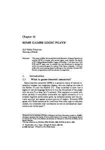
Now we can analyze the lexical predicate “to kill”; the meaning of the word “kill” is represented by a semantic-cognitive scheme (Descl´es, 1990) illustrated by the following λ-expression: (29)
“to kill” =def λy.(λx.(T RANS-CHANGI (SIT T1 [y])(SIT T2 [y]))x)) 1 (to be-alive z)))y with: SIT T1 [y] = (λz.(ST AT EO 2 (Neg(to be-alive z)))y SIT T2 [y] = (λz.(ST AT EO and the constraints on topological intervals: [O1
Comments: The actor x of the event assumes a grammatical role of an agent. Being an agent, he “controls” and “carries out” the change (CHANG) that turns the static situation SIT1 into a static situation SIT2 . The operator TRANS — in the sense of “semantic transitivity” — expresses the integration of the two operators, one is the “control” (CONTR) and the second one is the “execution” (DOing) which are closely related to an agentive role (see Descl´´es, 1990) assumed by a term in a predicative relation. The two situations SIT1 and SIT2 concern the same patient y which undergoes the change. The interval O1 , on which the situation SIT1 is realized, precedes the interval O2 , on which the situation SIT2 is realized. As both of the two intervals are open, they are necessarily separated by a closed interval I which shares the common boundaries: the left boundary γ(I) of I is identical to the right boundary δ(O1 ) of O1 , the right boundary δ(I) of I is identical to the left boundary γ(O2 ) of O2 . The change that y undergoes is therefore actualized on the interval I, which is nested between the two intervals O1 and O2. : the intitial static situation SIT1 was actualized on the interval O1 and the final situation SIT2 will be actualized on the interval O2 . We represent the intrinsic meaning of “to kill” by a temporal diagram given in figure 6. O1
]
[<
I
>]<
O2
>[
<- - - the deer is alive - - ->EVEN I (the hunter kills the deer)<- - the deer is no longer alive - ->
Figure 6.
From the statement: (30)
&{P ROCJ0 (SAY((this morning)O3 (EV EN NF1 (to kill a-deer the-hunter))S 0 )} {&([δ(F 1 )<γ(J0 )])([O3 ⊃ F 1 ])([O3 <J0 ])}
we deduce, by means of an integrative process, that the event (31)
(EV EN NF1 (to kill the-deer the-hunter))
was actualized at the right boundary δ(F1 ) of the interval F1 which precedes the interval J0 of actualization of the utterance. We are also going to deduce that the state:
234
LOGIC, THOUGHT AND ACTION (32)
((now)0J )(ST AT EJ0 (to be-dead the-deer))
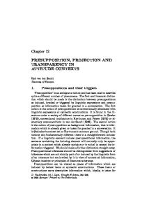
is true on the interval J0 . We take a synchronized diagram to represent the temporal intervals of the underlying situation of sentence (26a. We are now going to present a formal proof of the previous inference (26a, b). To simplify the notations, we use the symbols T1 for “the hunter” and T2 for “the deer”. The initial statement with the constraints on the temporal intervals is: (33) (P ROCJ0 (SAY((this morning)O 3(EV EN NF1 (P P2 T 2 T 1 )))S 0 ) 1 0 3 1 with the coordonates: [d(F )
So we have a nested event which is actualized on the interval F1 which occurred before the speech-act and this event is inside the temporal interval O3 defined by “this morning”, hence the conditions on intervals: [d(F1 ) < g(J0 )] (“F1 before the speaking act”); [ O3 ⊃F1 ] (”F1 is inside the interval O3 defined by “this morning”); [O3 < J0 ] (“this morning” is located before the speaking act”). Comments on deduction I: Expression (33) introduces the declarative hypothesis. This declaration allows us to actualize predicative relations on intervals. The underlying predicative relation is true on a closed interval F1 which precedes the interval J0 of speech-act. From this hypothesis, one can assert that the event has occurred on an interval F1 (step 1). Step 2 defines the meaning of “to kill” by a λ-expression. This meaning is used to decribe the lexical meaning of the event. Then follow the substitutions of arguments in the places linked by the abstraction operator λ, which leads to step 6. This result brings about a unification of intervals : the interval F1 becomes the actualization interval of the event “killing”, therefore [I = F1 ] (step 8). As the event is completely actualized on the interval F1 , we deduce that the final situation SIT2 of the event is actualized. This final situation is part of the meaning of the predicate “to kill”, so it is actualized on the open interval O2 which is adjacent to F1 (step 9). Topological consideration on order of instants concerning the intervals justify the following reasoning (step 10): since F1 is nested between the two adjacent states O1 (before F1 ) and O2 (after F1 ), and since O3 includes F1 (initial hypothesis) and O3 precedes J0 , we can deduce that O3 has a non-empty intersection with O2 . By contiguity of intervals in the same referential framework, we deduce that O2 includes J0 ; it follows that the two right boundaries of O2 and of J0 must be actualized at the same instant, hence the two right boundaries are identical. Since the state is true on the interval O2 and the interval O2 includes the interval J0 , it follows (property of states) that the same state has to be true on the interval J0 (step 11). Step 12 asserts a lexical equivalence between the one-place predicate “be-dead”
235
Reasoning and Aspectual-Temporal Calculus
Deduction I: 1.
(this morning)O3 )(EV EN NF1 (to kill T 2 T 1 )) 3 1 [O ⊃ F ] [O3 < J 0 ] [F 1 < J 0 ]
2.
[to kill=def Λy.(Λx.(TRANS-CHANGI (SIT1 [y])(SIT2 [y]))x))] def. “to kill”
3.
EV EN NF1 (Λy.(Λx.(TRANS-CHANGI (SIT1 [y])(SIT2 [y]))x)T 2 T 1 ) repl. 1, 2
4.
EV EN NF1 ((Λx. (TRANS-CHANGI (SIT1 [T 2 ])(SIT2 [T 2 ]))x)T 1 ) reduction, 3
5.
EV EN NF1 (TRANS-CHANGI (SIT1 [T 2 ])(SIT2 [T 2 ]))T 1 )
6.
1. 2. 3. 4.
2
SIT1 [T ] SIT1 [T 2 ] SIT2 [T 2 ] SIT2 [T 2 ]
= = = =
1 (Λz. (ST AT EO (to be-alive z))) 1 ST AT EO (to be-alive T 2 ) 2 (Λz. (ST AT EO (Neg(to be-alive 2 ST AT EO (Neg(to be-alive T 2 ))
hyp. hyp. hyp. hyp.
T
2
z)))) T 2
7.
1 EV EN NF1 (TRANS-CHANGI (ST AT EO (be-alive T 2 )) 2 2 (ST AT EO (Neg(be-alive T ))) T 1 )
8.
[O1 < F 1 < O 2 ] [δ(O1 ) = γ(F 1 )] [γ(O2 ) = δ(F 1 )]
9.
2 ST AT EO (Neg(to be-alive T 2 )) from 7
reduction, 4 def. SIT1 reduction,6.1 def. SIT2 reduction,6.3 repl. 5, 6.2, 6.4 unification F 1 /I with [I = F 1 ]
[O1 < F 1 < O 2 ] [O3 ⊃ F 1 ] [O3 < J 0 ] [O3 ∩ O2 �= ∅] [O2 ⊃ J 0 ] [δ(O2 ) = δ(J 0 )]
10.
1. 2. 3. 4. 5. 6.
11.
ST AT EJ0 (Neg(to be-alive T 2 ))
from 9, 10.5
12.
[to be-dead =def B Neg(to be-alive)]
def.
13.
ST AT EJ0 (to be-dead T 2 ) repl.,
int. B, 11, 12
from 8 initial hyp. initial hyp. from 1, 2 from 1, 2, 3, 4 from 5
14.
BST AT EJ0
15.
[PRST-STATE =def BST AT EJ0 ]
def.
16.
[prest-state =def PRST-STATE ]
def. of prest
(to be-dead) T
2
2
17.
prest-state (to be-dead) T
18.
[is-dead =def prest-state (be-dead)] 2
int. B, 13
repl., 14, 15, 16 def
19.
[T : = the-deer]
instantiation of T 2
20.
is-dead the-deer
repl. 17, 18, 19
236
LOGIC, THOUGHT AND ACTION
and the composition (by the combinator B) of the propositional negation, noted “Neg”, with the predicate “be-alive”. After the substitution, we obtain step 13. Step 14 is the result of the composition of the aspectual operator with the lexical predicate “be-dead”. Step 15 defines the grammatical operator PRST-STATE. Step 16 defines the morphological predicate prest-state (“present state”) as being the morphological trace of the grammatical operator PRST-STATE. Step 17 is the result of the replacement. Step 18 is the definition of a tensed and aspectualized lexical predicate. Step 19 is an instantiation of the variable T2 , hence the applicative expression at step 20. Finally, we have the relation of inference: (34)
(P ROCJ0 (SAY (EV EN NF1 (to kill the-deer the-hunter))S 0 ) →β 1 EV EN NF (to kill the-deer the-hunter)→β ST AT EJ0 (Neg(to be-alive) the-deer)→β ST AT EJ0 (to be-dead the-deer)
this means, at the level of configurations of the phenotype level: (35)
6.
I say that the hunter killed the deer → The hunter has killed the deer → The deer is not alive→ The deer is dead
Other Examples of Inferences Let us now examine a more complex reasoning:
(36)
a. b. c. d.
This morning, the hunter killed the deer therefore the deer was killed (this morning) therefore the deer is (at the moment)no longer alive therefore before this morning, the deer was alive
In the same way, we represent several inferences by formalized deductions. (37)
This morning, the hunter killed the deer → The deer was killed
Comments on Deduction II: the hypotheses are given in step 0: the interval O3 related to this morning includes the event realized on F1 which precedes J0 . This event actualized on F1 generates a “passive event” actualized on F2 where F2 is concomitant with F1 . The “passive predicate” (see the next remark) is derived from the active predicate. So, for the active predicate “to kill”, there is the associated passive predicate “to be killed”. However, while the agent T1 is explicit in the active
237
Reasoning and Aspectual-Temporal Calculus Deduction II: 0.
P ROCJ0 (SAY (EV EN NF1 (to kill T 2 T 1 ))S 0 ) [O3 ⊃ F 1 ]&[F 1 < J 0 ]&[O3 < J 0 ]
hyp.
1.
EV EN NF1 (to kill T 2 T 1 )
from 0
2.
EV EN NF2 (P ASS 2 0
(to kill)) T
2
[F < J ]
3.
BEV EN NF2 P ASS (to kill) T 2
4.
[past-passive=def BEV 2
EN NF2 P ASS]
passive predicate, 1 unification [F 2 = F 1 ] int. B,2 def. past-passive
5.
past-passive (to kill)T
6.
[was-killed=def past-passive (to kill)]
def.
repl. 3, 4
7.
[T 2 := the deer ]
instantiation of T 2
8.
was-killed the-deer
repl. 5,6,7
form, it remains implicit in the short passive form. Step 3 introduces the combinator B which allows us to compose the aspectual operator with the passivization operator PASS. In step 4, the definition of the grammatical operator “past-passive” is given, which leads to the passive lexical predicate was-killed in step 6. After substitution, we obtain the step 8 which represents the passive sentence the deer was killed, that is actualized on the interval F2 concomitant with F1. This latter event presents an occurrence inside the interval defined by O3 (this morning). Remark: We have presented an analysis of the passivization in the theoretical framework of Applicative Grammar (see: Descl´´es (1990), Guentcheva, ´ Shaumyan (1985) and Descl´ ´es & Guentch´eva (1993)). The basic structure of the passive is a “short” construction, which means “agentless” with an intransitive “passive predicate”. The passive predicate is constructed on the basis of the active one. The analysis uses the combinator of conversion C and also the existential quantifier noted “Σ”: [Ppass =def Σ(CPactive )]. From the “short” passive construction Ppass T, we deduce with the presence of a term denoting a “non-specified agent” x1 — expressed in French by “on” -, according to a classic elimination rule of the quantifier Σ in natural deduction: Pactive T x1 . In this way, we have the reduction of the passive construction (for example: the deer was killed ) to its active equivalent (for example: one killed the deer ): In this way, the explicit definition of the grammatical operator of the passivization PASS is in order. (38)
The deer was killed this morning → The deer is not alive
Comments on deduction III: we start with the passive predicate (the deer was killed, this morning) and the conditions on the intervals.
238
LOGIC, THOUGHT AND ACTION 1. 2. 3. 4. 5.
Ppass T [Ppass = Σ(CPactive )] (Σ(CPactive ))T (CPactive ) x1 T Pactive T x1
hyp. passive predicate repl. 2., 1. elim. Σ, 3. elim.C, 4.
Deduction III: 1.
EVEN2F (PASS (to kill)) T2 [ F 2 < I0 ] [ O3 ⊃ F 2 ] [ O3 < I0 ]
2.
[to kill =def λy.(λx.(TRANS-CHANGI (SIT T1 [y])(SIT T2 [y]))x))]
passive event
EN NF2 (λy.(λx.(TRANS-CHANGI (SIT T1 [y])(SIT T2 [y]))x)T 2 x1 )
def.
3.
EV [ x1 = non-specified agent ]
4.
EV EN NF2 (P ASS(TRANS-CHANGF 2 unification[I=F 2 ] 1 2 ((to be-alive)T 2 ))(ST AT EO (Neg((to be-alive)T 2 )x1 )) from 3 (ST AT EO [O1
5.
2 ST AT EO (Neg(to be-alive)T 2 )) [ O 2 ⊃ J0 ] [ δ(O2 ) = δ(J0 )]
6.
ST AT EJ0 (Neg((to be-alive) T 2 ))
7. 8.
2
B
ST AT EJ0
Neg(to be-alive) T 2
[ not-be-alive =def B 2
9.
[ T = the-deer ]
10.
not-be-alive the-deer
repl., 1, 2,
from 4
from 5
2
ST AT EJ0 N eg(to
int. B2 be-alive)]
def. instantiation of T2 from 8, 9, 10
We introduce the definition of the lexical predicate “to kill” in step 2. After the reductions, the result shows that the event has been actualized on the closed interval F2 which is nested between the two open intervals O1 and O2 (step 4). We obtain the conclusion that the final state of the event is actualized on the interval O2 : the negation of “T2 is alive” is true on O2 . A reasoning about the intervals shows that the intervals O2 and J0 have the same right boundary. According to the property of states which stipulates that the state is actualized on O2 and that O2 includes J0 , we conclude that the state is actualized on J0 (step 6). The introduction of the combinator B2 allows us to define, in step 8, the complex static predicate “not-be-alive”. Finally, after replacement, we get step 10. (39) The deer was killed this morning → The deer was alive before this morning
239
Reasoning and Aspectual-Temporal Calculus Deduction IV: 1.
EV EN NF2 (P ASS(tokill))T 2 [ F 2
2.
EV EN NF2 (P ASS(TRANS-CHANGF 2 unification[I=F 2 ] 1 2 ((to be-alive)T 2 ))(ST AT EO (N eg((to be-alive) T 2 )))x1 )) ST AT EO passive reductions [ x1 = non-specified agent ] unification [ O1
3.
1 ST AT EO ((to be-alive) T 2 ) 3 1 [ O ∩ O �= ∅ ]
4.
[ [ [ [
5.
ST AT EO�� ((to be-alive) T 2 ) [ O�� <J0 ]
6.
BST AT EO�� (to be-alive)T 2
7.
passive event
from 2
O� =def O1 − O3 ] O� ⊃ O�� ] O��
def. of O’
from 3 int.B, 5 ��
[ past-state =def &(BST AT EO�� )([O <J ]) 0
def. of past state
8.
[ was-alive =def past-state (to be-alive)
9.
[ T 2 : = the-deer ]
instantiation of T 2
def.
10.
was-alive the-deer
from. 6, 7, 8
Comments on deduction IV: We start from the passive sentence that represents an actualized event on the interval F2 which is nested in the interval O3 associated with this morning. The meaning of the lexical predicate “to kill” enables us to deduce step 2, with x1 denoting a non specified agent implied by a passive construction. Since the event is actualized on F2 , it follows that the initial state has been actualized on the interval O1 which precedes the interval F2 and is adjacent to it (step 4). We define the interval O’ as being before the interval O3 . As the state “T2 to be alive” was actualized on the interval O1 , it is actualized, according to the property of states, on the interval O’, nested in O1 . Hence step 5. The introduction of the combinator B in step 6 enables us to define the morphological operator past − state in step 7, hence the complex predicate “was-alive” in step 8. After the instantiation of T2 we finally obtain the applicative expression at step 10.
240
7.
LOGIC, THOUGHT AND ACTION
Final Remarks
The above reasonings show how we can relate sentences by means of oriented inferences. Several remarks are now in order: 1) It has been shown how we can formalize the inferential reasonings that are inherent in natural languages by means of aspectual-temporal conditions on the one hand and by means of representations of verbal meanings on the other hand. In this article, we have only illustrated this formalism by a few sentences. However, the other sentences given in the Introduction can be analyzed in the same manner. To formalize those sentences, one would need to introduce other notions, especially the notion of different referential spaces (for speech-act, for narrative texts and for counter-factual events. . . ). 2) The calculus introduced in this article has not been entirely formalized. In order to do this, one would need to better specify the semantics of the topological intervals, the rules on the inter-relations of temporal intervals (Allen’s calculus on intervals is clearly not sufficient since it does not take into account the topological bounds) and the relations between states, events and processes. In paragraph 2, we have formulated several rules but more rules need to be added. Furthermore, since the demonstration of Gentzen’s natural deduction has been slightly extended in this article, we would need to specify the formal conditions of such an extension. 3) We do not think and have not claimed that the speaker who produces these sentences has to call upon the aspectual-temporal operational processes that have been presented in this article. Yet, the nature of the encountered problem shows the complexity of information representation and processing. There may be a completely different calculus strategy to resolve and control the concrete subject of the analysed sentences. What has been presented in this article is simply a frame of one operational solution.
Appendix: Combinatory Logic We consider (see Descles, 1990), S.K. Shaumyan (1987) and other linguists that combinatory logic is very useful for analysing the meaning of grammatical operations and the meaning of lexical predicates. The aim of the Combinatory Logic (Curry, 1958) is operational processings by which operators — either elementary or complex — apply to operands. In general, operators and operands are of different types. However, we have not used this notion of type here. The basic constitutive operation of the expressions is called application. An expression that is constructed by the application is called applicative expression. An operator X that applies to an operand Y produces a result Z. We note the result of the application of X to Y by a simple concatenation which prefixes the operator to its operand, so: Z = XY. We stipulate: XYZ = def (XY)Z. It is evident that XYZ �= X(YZ).
241
Reasoning and Aspectual-Temporal Calculus
Some of the abstract operators, called combinators, are especially employed to construct complex operators from more elementary ones. The operational action of a combinator (see Fitch, 1974) is given by an introduction rule and an elimination rule, in Gentzen’s “natural deduction” style. We will give two examples: the first is the combinator B that represents the “functional composition” of operators which would be the expressions of set functions. Its operational action is defined by the two rules: 1. 2.
X(YZ) BXYZ
int. B
1. 2.
BXYZ X(YZ)
elim. B
The operational action of the combinator C of “conversion” is defined by the two rules: 1. 2.
XZY CXYZ
int. C
1. 2.
CXYZ XZY
elim. C
The third combinator that we introduce here is the combinator of identity I. The rules are as follows: 1. 2.
X IX
1. 2.
int. I
IX X
elim. I
Starting from the basic combinators (very small in number), one can generate, by means of the operation of application, an unlimited number of derived combinators. For example, for the combinator B2 , derived from the combinator B, one has the definitional relation: [B2 =def BBB ]. Its operational action is deduced by the successive introductions or eliminations of B: Introduction of B2 1. 2. 3. 4. 5. 6.
X(Z1 Z2 Z3 ) BX(Z1 Z2 )Z3 B(BX)Z1 Z2 Z3 BBBXYZ1 Z2 Z3 [B2 =def BBB ] B2 XYZ1 Z2 Z3
Elimination of B2 1. 2. 3. 4. 5. 6.
B2 XYZ1 Z2 Z3 [B2 =def BBB ] BBBXYZ1 Z2 Z3 B(BX)Z1 Z2 Z3 BX(Z1 Z2 )Z3 X(Z1 Z2 Z3 )
From this we deduce the two relations of β-expansion (←β ) and of β-reduction (β →): X(Z1 Z2 Z3 ) ←β B2 XYZ1 Z2 Z3
B2 XYZ1 Z2 Z3 β → X(Z1 Z2 Z3 )
A combinator represents an applicative program of construction of a complex operator from more elementary operators. Therefore, the combinator B2 combines the operators X and Y in a way to apply the complex operator (B2 XY) successively to the operands Z1 , Z2 and Z3 , and this gives the result: X(Z1 Z2 Z3 ). An applicative expression that cannot be further reduced is called a normal form. For example, X(Z1 Z2 Z3 ) is a normal form associated with the applicative expression B2 XYZ1 Z2 Z3 . Let X and Y be any two applicative expressions. We stipulate:
242
LOGIC, THOUGHT AND ACTION X 0 Y = BXY
The composition ‘0’ between two operators is associative. We have for example: B2 = B O B = BBB I=C0C
References Abraham M., (1995): Repr´ ´esentation s´emantique des verbes (verbes de mouvement) en vue d’un traitement informatique, Ph.D. Dissertation, Universite´ de Paris-Sorbonne, March 1995. Allen J., (1983): “Maintaining Knowledge About Temporal Intervals”, Communications of the ACM, 26, 832–843. Benveniste E. (1964). Problemes ` de linguistique g´ ´en´ ´rale . Paris: Gallimard Bertinetto P.M., Bianch V., Higginbotham J., Squartin M. (eds.), (1995). Temporal Reference Aspect and Actionality. Turin: Rosenberg & Sellier Comrie B. (1976): Aspect, an Introduction to the Study of Verbal Aspect and Related Problems. London: Cambridge University Press. Culioli A. (1990). Pour une linguistique de l’´ ´enoncation, op´ ´rations et repr´sentations ´ . Paris: Ophrys Curry H., (1958). Combinatory Logic. Amsterdam: North Holland. David J. & Martin R. (1980). Notion d’aspect. Paris: Klincksieck. Descles ´ J.-P. (1980): “Construction formelle de la cat´ ´egorie de l’aspect (essai)”, in David & Martin Notion d’aspect, 198–237. Paris: Klincksieck. — (1990a). Langages applicatifs, langues naturelles et cognition.. Paris: Herm`es. — (1990b): “State, Event, Process, and Topology”, in General Linguistics, 29, 3:159–200. University Park and London: Pennsylvania State University Press. — (1991). “Arch´ ´etypes cognitifs et types de proc``es”, Travaux de linguistique et de Philologie, XXIX: 171–195. — (1993). “Remarques sur la notion de processus inaccompli”, S´mioti´ que, 5 , December 1993, 31–55. Paris: Didier-Erudition. — (1994). “Quelques concepts relatifs au temps et `a l’aspect pour l’analyse des textes”, in Descl´es et alii (1994), pp. 57–88. — (1994). “Relations casuelles et sch``emes s´emantico-cognitifs”, Langages, 113, 113–125. — (1997). “Logique combinatoire, topologie et analyse aspecto-temporelle”, in Descl´es et alii, pp. 37–69. Descles, ´ J.-P., Guentch´eva, Z., Shaumyan S.K. (1985). “Passivization in Applicative Grammar”. Pragmatics & Beyond VI, I 1. John Benjamins.
Reasoning and Aspectual-Temporal Calculus
243
Descles ´ J.-P., Guentch´eva Z. (1990). “Discourse Analysis of Aoriste and Imperfect in Bulgarian and French”. Verbal Aspects. Amsterdam : Thelin, Benjamins. Descles, ´ J.-P., Guentch´eva, Z. (1993). “Le passif dans le syst``eme des voix du fran¸cais”. Langage, 109, 1993, 73–102. Paris: Larousse. Descles ´ J.-P., Guentch´eva Z., Karolak S., Koseka-Toszewa V. (1994). Studia Kognitywne, T.1: Semantyka kategorii aspektu i czasu. Warszawa: Slawistyczny Osrodek Wydawnczy. Descles ´ J.-P., Guentch´eva Z. (1995). “Is the Notion of Process Necessary?”. International Conference on Aspect, Cortona, October 9–12, 1993, in Bertinetto et alii, 55–70. Descles ´ J.-P., Guentch´eva Z., Karolak S., Koseka-Toszewa V. (1997). Studia Kognitywne, T.2: Semantyka kategorii aspektu i ezasu. Warszawa. Slawistycny Osrodek Wydawnczy. Descles ´ J.-P., Guentch´eva Z. (1997). “Aspects et modalit´´es d’action (Repr´ ´esentations topologiques dans une perspective cognitive”, in Descl´es et alii, 145–173. Descles ´ J.-P., Jouis C., Oh H.G., Reppert D. “Exploration contextuelle et semantique ´ : un syst` `eme expert qui trouve les valeurs s´ ´emantiques des temps de l’indicatif dans un texte”, in Knowledge modeling and expertise transfer 1991, 371–400, D. Herin-Aime, R. Dieng, J.-P. Regourd, J.-P. Angoujard (eds). Amsterdam, Washington DC, Tokyo: IOS Press. Dowty, D.(1979). Word Meaning and Montague Grammar. Dordrecht: Reidel. Fitch F. B. (1974). Elements of Combinatory Logic. New Haven: Yale University Press. ´ Z. (1990). Temps et aspect : l’exemple du bulgare contempoGuentcheva rain. Coll. Sciences du langage, Paris: Editions du CNRS. Kamp H. (1981). “Ev´ ´enements, repr´´esentations discursives et r´´ef´ ference temporelle”, Langages 64, 39–64. Kamp H. & Rohrer C., (1983). “Tense in texts” in R. Bauerle et alii (ed.), Meaning, use and interpretation of language. Berlin: de Gruyter, 250–269. Karolak S. (1997). “Le temps et le mod``ele de H. Reichenbach”, in Descl´es J.-P., Guentcheva ´ Z., Karolak S., Koseka-Toszewa V., (eds.) (1997), 95–125. Koseka-Toszewa V. & A. Mazurkiewicz (1994). “Description de la temporalit´ ´e et de la modalit´e au moyen de r´ ´eseaux” in Descl´es et alii, 89–112. Lyons J.(1977). Semantics, Vol. 2. London, New York, Melbourne: Cambridge University Press.
244
LOGIC, THOUGHT AND ACTION
Maire-Reppert D. (1990). Repr´ ´esentation des valeurs s´ ´emantiques de l’imparfait fran¸c¸ais en vue d’un traitement informatique , Ph.D. Dissertation. Universit´ ´e de Paris-Sorbonne. Maire-Reppert D., Oh H.G., Berri J. (1991). “Traitement informatique de la cat´ ´egorie aspecto-temporelle”, in T.A. Informations, 32, 1:77– 90. Mourelatos A. (1981). “Events, Processes and States”, in Tedeschi et Zaenen (eds), 192–212. Oh-Jeong H.G. (1991). Repr´ ´esentation des valeurs s´emantiques du pass´ compose´ fran¸cais ¸ en vue d’un traitement informatique . Ph.D. Dissertation. Universit´ ´e de Paris-Sorbonne. Prior A. (1967). Past, Present and Future. Oxford: Clarendon Press. Reichenbach H., (1947). Elements of Symbolic Logic. Toronto: The Macmillan Company. Searle J.R., Vanderveken D., (1985). Foundations of Illocutionary Logic. Cambridge University Press Shaumyan S. K. (1987). A Semiotic Theory of Language. Bloomington: Indiana University Press Smith C.S. (1991). The Parameter of Aspect. Dordrecht: Kluwer Academic Publishers. Thelin N.R. (1990). Verbal Aspect. Amsterdam, Philadelphia: John Benjamins. Vanderveken D. (1991). Meaning and Speech Acts, volume II Formal Semantics of Sucess and Satisfaction. Cambridge University Press Vendler Z.(1967). Linguistics and Philosophy. Ithaca, New York: Cornell University Press Vet C. (1995). “The Role of Aktionsart in the Interpretation of Temporal Relations in Discourse” n in Bertinetto et alii (1995), 295–306